Everyone makes inferences, general statements drawn from specific evidences or experiences, as they learn about and act in the world around them. Inferential statistics are powerful tools for making inference that rely on frequencies and probabilities. Consequently, an understanding of inferential statistics can improve one’s ability to make decisions, form predictions, and conduct research. It can also protect one from the misused and misinterpreted statistics that are all too common occurrences.
This chapter is not meant to teach all statistical principles or to convince the skeptic of the value of quality statistical inference. Instead it is meant to provide a brief taste of inferential statistics, just enough to help the reader decide whether or not to pursue more information on the topic. Three general topics will be covered in the chapter: (1) the importance of a representative sample, (2) the types of questions that can be answered by statistics, and (3) the most common branch of statistical analysis, which is called Null Hypothesis Significance Testing (NHST).
Sampling
We make inferences when we do not have access to the whole picture. For example, a candy company may want to be certain of the quality of their candies, so they taste a few. It is ludicrous to expect the company to taste all of their candies, because they would no longer have anything to sell. However, when they say that a whole batch is good or bad based on a sample, they are wading into uncertain territory. The same is true in inferential statistics. The process of inferential statistics has been labeled, “decision making under uncertainty” (Panik, 2012, p. 2). To reduce uncertainty it is necessary for the sample to represent the population (the whole batch of candies in this case). If the sample is not representative, then the inferences drawn about the population would be incorrect.
Theoretically, the best way to get a representative sample is called simple random sampling (SRS). Simple random sampling means that every person in the population, or every candy in the batch, has an equal chance of being selected. In practice this is often difficult or impossible. Researchers cannot force people to participate in their studies, so they are automatically limited to those who are interested in the study in the first place. With many other limitations preventing a truly random sample, many other options become necessary. These quasi-experimental designs tend to be complicated, leading some researchers to gather whatever sample is convenient. However, convenience sampling is not a good practice, and it greatly increases the chance of a non-representative sample, which invalidates the generalizability of the research. Instead, the aspiring researcher should familiarize himself or herself with the more complex quasi-experimental designs.
Statistical Questions
Foundational to the design of the experiment or study is the selection of the research question. The selection of the question leads naturally into the selection of an analysis and therefore requirements on the data that can and should be gathered.
Many different types of analyses are available, and each one lends itself to a different type of question or set of questions. A regression, for example, will tell you how strong the relationship is between one variable of interest and another. It will also tell you if one variable predicts the other and helps you make predictive models. A simple t-test will tell how probable it is for one group to be different from another. While each test may answer different questions, it is important to consider that all statistical analyses share one limitation in particular. Inferential statistics can only answer questions of how many, how much, and how often.
This limit on the types of questions a researcher can ask comes, because inferential statistics rely on frequencies and probabilities to make inferences. Consequently, only certain types of data may be used: nominal, ordinal, interval, or ratio (Panik, 2012, p. 4).
Nominal data consists only of a classification into groups, such as male or female, or control group or experimental group. Ordinal data is also categorical in nature but includes an order placed on the data. For example, first and second place in a race tell us nothing about the relationship between the two runners other than the fact that the first place runner came before the second.
Interval data and ratio data are very similar to each other and are often grouped together under the terms numerical or quantitative data. Interval data are like temperature in degrees Celsius. They are numbers that have meaning, but the zero is not an absolute zero. In the case of degrees Celsius, a zero does not mean a complete lack of temperature. It just means the point where water freezes. The temperature scale of Kelvins is different. Zero on that scale means absolutely no heat, making this scale a ratio scale.
Ratio data is often, but not always, the ideal data for an analysis. However the best way to determine what type of data to gather goes back to the research question. The research question will not only help you decide if statistics will help you, but it will also help you decide what type of data you should gather.
Null Hypothesis Significance Testing
Most people who have read an academic article have been exposed to something called a p-value. The p-value is fundamental to the most common statistical practice today, Null Hypothesis Significance Testing (NHST). NHST involves estimating the probability that the average of your sample is different from some other expected value (the null hypothesis). This probability estimate is the p-value. For example, if a researcher was investigating whether or not two groups were different, the null hypothesis would be “the difference between group A and group B is zero.” If the difference between the groups was 3.7, and the p-value was .03, then there would be a 3% chance that the difference in our sample was 3.7 if the true difference was zero.
For the novice statistician this can seem like a bit of a black box. When examined fully, however, it is not too hard to understand. The whole process involves giving the null hypothesis a score based on how many standard deviations away from the sample mean it is. The p-value is calculated from this score, and if the p-value is below a preset value (usually .05), then we say that it is “significant.”
Airline Example
To better clarify the process associated with many statistical inferences, consider the data in Table 1 (R Core Team, 2016).
Table 1. Airline Passenger Data
| 1959 | 1960 | Difference |
|---|
| 360 | 417 | 57 |
| 342 | 391 | 49 |
| 406 | 419 | 13 |
| 396 | 461 | 65 |
| 420 | 472 | 52 |
| 472 | 535 | 63 |
| 548 | 622 | 74 |
| 559 | 606 | 47 |
| 463 | 508 | 45 |
| 407 | 461 | 54 |
| 362 | 390 | 28 |
| 405 | 432 | 27 |
This is the number of passengers that flew each month on a certain airline in 1959 and 1960, as well as the differences between the two. A researcher may want to know if there was a difference in passengers between the two years. This researcher would first need to clarify the null and alternative hypotheses and set the alpha level (the level our p-value has to be before we will believe the conclusions).
H0: The average of 1959 = the average of 1960. (i.e the difference = 0)
Ha: The average of 1959 ≠ the average of 1960. (i.e the difference ≠ 0)
α = 0.05
In other words, the researcher is assuming the two are the same but will have enough evidence to support that they are different if the p-value is less than 0.05.
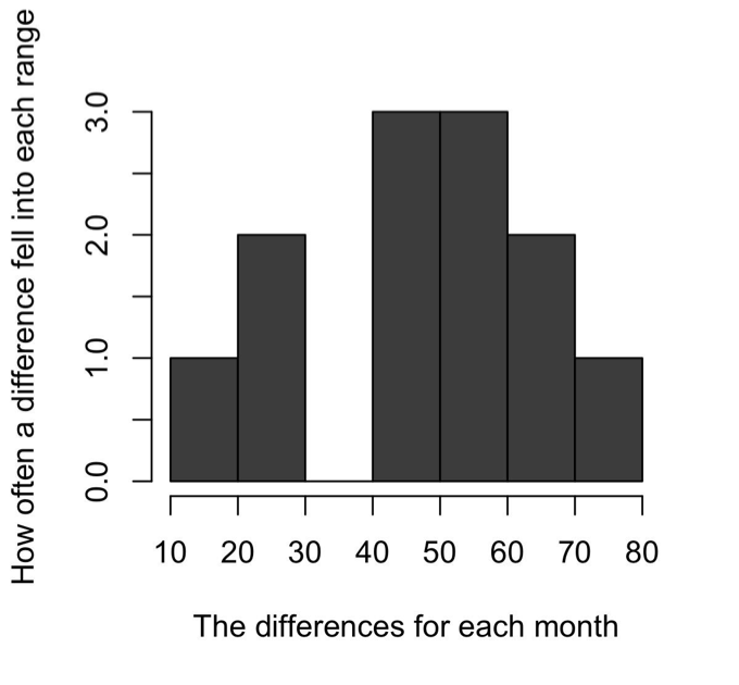
The differences between the two groups is found in column three. Our first step is to find the mean of this column by adding all of the values and then dividing by the number of data points we added together. This gives us a mean of 47.83. This sample mean is a point estimate, or an approximation, of the true difference. We know this data follows a certain pattern (Figure 1), called a normal distribution.

Fig. 1. Patterns of the Differences
Consequently, we know that 68% of the data is within one standard deviation, and 95% is within two standard deviations. A standard deviation is a measure of uncertainty. It is the average distance between the data points and the sample mean. We calculate the standard deviation using this formula (Moses, 1986, p. 50):

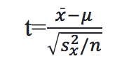
The standard deviation for the airline data is 17.58. A test statistic is obtained using the following formula (Vaughan, 2013, p. 47):

The test statistic for the airline question is 9.425. The p-value is the probability of getting a test-statistic as extreme or more extreme than the one you got, given the null hypothesis is true (Brase & Brase, 2016, p. 425). In other words, it is the probability of getting 47.83 as the average distance if the true average difference was 0. With a p-value of 0.000013, which is less than the .05 standard the researcher set at the start, there is enough evidence to reject the null hypothesis. Thus, the researcher concludes that there is a difference between the two groups. It is important to note that conclusions based on p-values alone lead to an incorrect answer 5% of the time. Consequently, it is good practice to interpret p-values in the context of other inferential statistics, such as effect sizes and confidence intervals. This approach is neither perfect, nor the only approach available, it is simply the most common.
Conclusion
Inferential statistics are an extension of the natural human tendency toward inference. They are powerful tools that can help answer questions such as how much, how many, or how often. An understanding of the process of statistics can help us be better consumers of research, prevent us from being misled by invalid or misinterpreted statistics, and give us another tool in the search for knowledge.
References
Brase, C. H., & Brase, C. P. (2016). Understanding basic statistics (7th ed.). Boston, Massachusetts: Cengage Learning.
Moses, L. E. (1986). Think and explain with statistics. United States of America: Addison-Wesley Publishing Company, Inc.
Panik, M. J. (2012). Statistical inference: A short course. Hoboken, New Jersey: John Wiley & Sons, Inc.
R Core Team (2016). R: A language and environment for statistical computing. R Foundation for Statistical Computing, Vienna, Austria. Retrieved from https://www.R-project.org/.
Vaughan, S. (2013). Scientific inference: Learning from data. Cambridge, United Kingdom: Cambridge University Press.
Keywords: inference, inferential statistics, null hypothesis significance testing