In this chapter, we're going to learn how to do sorting and filtering.
Practice Spreadsheet
Use this workbook for the chapter.
Note: This is the same workbook used in the Navigation Shortcuts chapter.
Sorting
Let's start with sorting. In our spreadsheet, we have a list with a header at the top. It always helps to have a header of labels at the top for sorting. To sort, do the following.
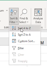 Figure 12.1
- Select all of the data in the list that we want to sort.
- Select the upper left-hand cell in the list.
- Control+Shift+Right, Control+Shift+Down to get the whole thing selected.
- On the right side of the Home tab, you will find the Sort & Filter option. (See Figure 12.1)
- If we select Sort A–Z, it will sort everything in ascending order by the first column selected. Z–A will go in descending order.
- If we know that we want to sort by the first column, then we can go ahead and use one of those two. But if we want to sort by another column, or by multiple columns, we select Custom Sort.
Custom Sorting
Let's suppose we want to do a little bit different sort. Once you have selected custom sort, you can select multiple levels of sorting. The box that opens starts with a single row, telling you that it will sort by the first column based on the order Z to A. (See Figure 12.2)
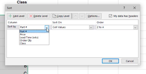 Figure 12.2
To add a level, choose to sort next based on any of the other columns that we have.
In this example, we’ll do the following.
- Change first to sort by our class, and sort it A to Z on our next level.
- On the next level, sort by price, this time from the largest to the smallest price.
- You’ll notice it recognizes that this column contains numbers because it switched the verbs in the order column.
- Select OK.
- You'll notice it now sorted the list based first on the class, next on the price.
- As you scroll down and get past the A section, you’ll begin to see the B section and eventually the C section, with all of those sorted with their prices from highest to lowest within that subset.
One other thing to note here is that when you do a custom sort, there is a check box here at the top of the box that appears that says My Data Has Headers. (See Figure 12.3)
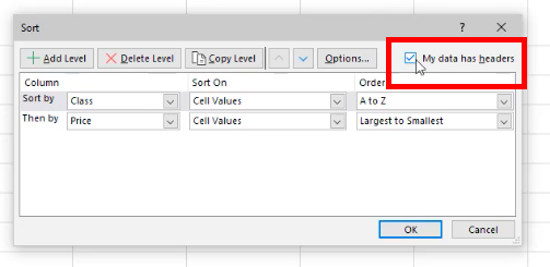 Figure 12.3
When this is selected, it means that there is a header row at the top, and it will automatically deselect that row. It also allows it to know what options should exist in the drop-down lists. If you deselect this, now it will include the top row in the sorting and it only does it by column. So, generally, it makes sense to have a header row, and then to checkmark that your data has a header row in it.
Data Filters
The second thing you will learn about is data filters. In order to turn on a filter, go onto the Home tab again. Off to the upper right-hand corner under Sort and Filter, select Filter. (See Figure 12.4)
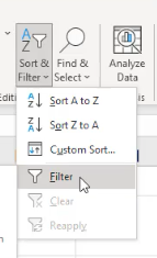 Figure 12.4
When you do this, it will recognize all of the data on the sheet and put a filter in place at the top. A filter is a series of drop-down lists that allows us to manage a table using those drop-down arrows. (See Figures 12.5 and 12.6)
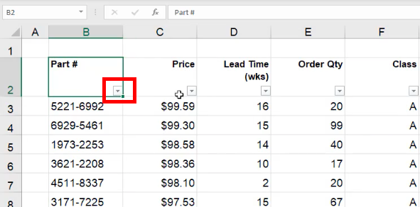 Figure 12.5
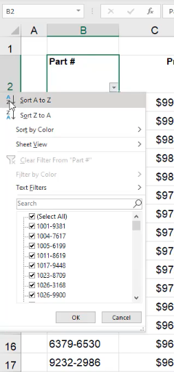 Figure 12.6
Instead of sorting, if you want, you can also filter out certain entries. By default, everything is selected. If you open up the drop-down arrow again, for example, in the Class column, when you uncheck the Select All box, nothing will be selected. Then, you can scroll down and select the items that you want to be sorted. (See Figure 12.7)
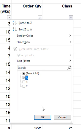 Figure 12.7
When you select OK, notice that it filters out everything in the list, except for the items that you had check marked. When something is filtered, a filter icon will replace the arrow icon that had previously been displayed. Only the items selected are shown in the list. Now, it's important to note that they're not gone. They're just hidden. You'll notice with the row that the numbers jump because the information that wasn’t selected is hidden.
In addition to the filter in the Class column, you could also add a filter to the Lead Time. This time, instead of checking things off the list, you can choose Number Filters, which provides many more different automatic filters. For example, you can select a Less Than filter, and show only items Less Than 10. (See Figure 12.8)
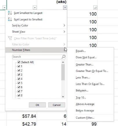 Figure 12.8
Why is this useful? Suppose you wanted to look at only the A items. With a filter, rather than having to scroll through thousands of items, you now can scroll through a much smaller and more specific list. Taking it a step further, if you added one more number filter to the Price column, you can select everything that’s less than ten dollars. Now, you only have 32 items that you can see very quickly and go through line by line if needed.
Removing Filters
To remove all these filters, you can individually go through and choose clear filter. Or, you can also go back to the Sort and Filter button in the top right, and choose Clear. This resets everything to the way it was prior to the filter being applied.
In addition, you can use the Control+Shift+L shortcut to add or clear filters, but to make sure all your data is included, it is recommended that you select all of the data before entering the shortcut.
 Figure 12.9